Data wrangling using data from AirBNB
![]()
This notebook applies the concepts we learned in class to an real dataset about current lists on AirBNB.
Manipulate and clean data
Data is often “dirty” and needs to be cleaned up before we can analyze it. Excel can do some of this but one limitation to Excel is that there is no audit trail for the transformations that have been applied to the data. This can lead to issues with reproducing the results later. It also leads to “magic numbers” which are values like 40 or 120 that appear in calculations but have no clear origin - they appear like magic and are hard to traceback to an origin.
Tutorial Overview
In this module, we will:
- import a file into a DataFrame
- remove extra characters in a column and recast the column as numeric
- plot the data as boxplots and histograms
- pivot ant cross-tabulate the data
- apply statistical techniques like ANOVA and regression to explore relationships in the data
We begin by importing pandas and numpy and reading in the dataset. Now we have a Pandas DataFrame with the data. You’ll notice this throws an error. Pandas automatically sets the data type for the columns during the import. Some of the columns are mixed which will create issues for our analysis.
! pip install -r requirements.txt

import pandas as pd
import numpy as np

df = pd.read_csv('data/AirBNB Toronto.csv')

# you can see the DataFrame is large - it has 106 columns.
# We won't need all of these so you could drop the columns you don't need.

df.head()
cols_to_drop = ['listing_url','scrape_id','last_scraped']
df.drop(cols_to_drop, axis=1, inplace=True)

# Let's look at the column for price. We want to see how the values are distributed.

df['price'].describe()
count      22425
unique       534
top       $99.00
freq         950
Name: price, dtype: object
# The "describe" method didn't seem to work. Let's try to plot 'price' using a boxplot and histogram. Why doesn't this work?
df.boxplot(column=['price'])
---------------------------------------------------------------------------

KeyError                                  Traceback (most recent call last)

<ipython-input-112-232150201d49> in <module>
      1 # The "describe" method didn't seem to work. Let's try to plot 'price' using a boxplot and histogram. Why doesn't this work?
----> 2 df.boxplot(column=['price'])


/opt/anaconda3/lib/python3.7/site-packages/pandas/plotting/_core.py in boxplot_frame(self, column, by, ax, fontsize, rot, grid, figsize, layout, return_type, **kwds)
    418         layout=layout,
    419         return_type=return_type,
--> 420         **kwds
    421     )
    422


/opt/anaconda3/lib/python3.7/site-packages/pandas/plotting/_matplotlib/boxplot.py in boxplot_frame(self, column, by, ax, fontsize, rot, grid, figsize, layout, return_type, **kwds)
    353         layout=layout,
    354         return_type=return_type,
--> 355         **kwds
    356     )
    357     plt.draw_if_interactive()


/opt/anaconda3/lib/python3.7/site-packages/pandas/plotting/_matplotlib/boxplot.py in boxplot(data, column, by, ax, fontsize, rot, grid, figsize, layout, return_type, **kwds)
    318             columns = data.columns
    319         else:
--> 320             data = data[columns]
    321
    322         result = plot_group(columns, data.values.T, ax)


/opt/anaconda3/lib/python3.7/site-packages/pandas/core/frame.py in __getitem__(self, key)
   2984             if is_iterator(key):
   2985                 key = list(key)
-> 2986             indexer = self.loc._convert_to_indexer(key, axis=1, raise_missing=True)
   2987
   2988         # take() does not accept boolean indexers


/opt/anaconda3/lib/python3.7/site-packages/pandas/core/indexing.py in _convert_to_indexer(self, obj, axis, is_setter, raise_missing)
   1283                 # When setting, missing keys are not allowed, even with .loc:
   1284                 kwargs = {"raise_missing": True if is_setter else raise_missing}
-> 1285                 return self._get_listlike_indexer(obj, axis, **kwargs)[1]
   1286         else:
   1287             try:


/opt/anaconda3/lib/python3.7/site-packages/pandas/core/indexing.py in _get_listlike_indexer(self, key, axis, raise_missing)
   1090
   1091         self._validate_read_indexer(
-> 1092             keyarr, indexer, o._get_axis_number(axis), raise_missing=raise_missing
   1093         )
   1094         return keyarr, indexer


/opt/anaconda3/lib/python3.7/site-packages/pandas/core/indexing.py in _validate_read_indexer(self, key, indexer, axis, raise_missing)
   1175                 raise KeyError(
   1176                     "None of [{key}] are in the [{axis}]".format(
-> 1177                         key=key, axis=self.obj._get_axis_name(axis)
   1178                     )
   1179                 )


KeyError: "None of [Index(['price'], dtype='object')] are in the [columns]"
# What is this histograph showing us?
df['price'].hist()
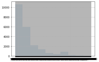
When Pandas imported ‘price’, it determined this variable was a string, not a number because it included the dollar sign and commas.
We need to remove “$” and “,” and then recast this column as a number (floating point since it has decimals). We can quickly fix the issues with price and continue our analysis. It is very common for datasets to have issues like this.
df['price'] = df['price'].str.replace('$', '')
df['price'] = df['price'].str.replace(',', '').astype(float)
# Now that we have the price as a number, we can make a boxplot.

df.boxplot(column=['price'])
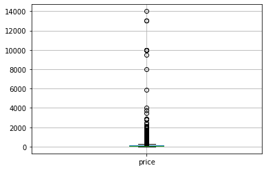
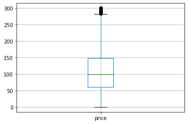
# The boxplot is hard to read because there are so many extreme values. Let's focus just on the values less than  or equal to $300.

df[df['price']<=300].boxplot(column=['price'])
# And we can make a histogram of the same distribution.

df[df['price']<=300]['price'].hist()
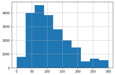
At this point, we might want to save the cleaned DataFrame as a CSV so we don’t need to repeat those steps. We have cleaned the price column, now let’s do some analysis.
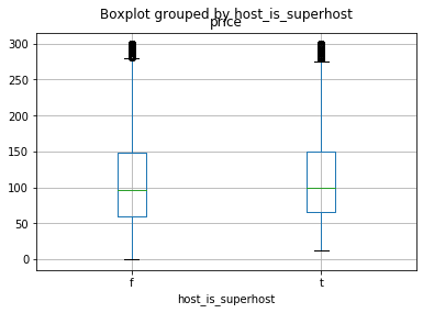
# We wonder if being part of the AirBNB "superhost" program is worth it. Let's look at the distribuition of rental prices separated by if the host is a superhost or not.

df[df['price']<301].boxplot(column=['price'], by = 'host_is_superhost')
# Adding a pivot table to look at the difference in price between superhosts and non-superhosts. The dataset uses "t" and "f" but lets change them to boolean values
bool_map = {'t': True, 'f': False}
df['host_is_superhost'] = df['host_is_superhost'].map(bool_map)

pd.pivot_table(df, values = 'price', columns = 'host_is_superhost', aggfunc='mean')
# We can use SciPy to test if the difference between superhosts/non-super hosts is statistically significant

from scipy import stats

stats.ttest_ind(df[df['host_is_superhost']==True]['price'], df[df['host_is_superhost']==False]['price'])
Ttest_indResult(statistic=0.14155977023038302, pvalue=0.88742901748445)
Conclusion
There is not evidence to indicate that the true mean rental price is different between superhosts and non-superhosts. (We fail to reject the null hypothesis.)
Bed_type and Price
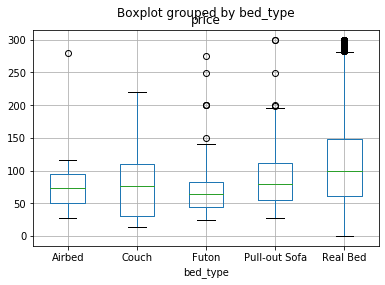
Let’s see if the kind of bed offered is correlated with price.
# Let's look at bed type and see if that makes a difference.

df[df['price']<301].boxplot(column=['price'], by = 'bed_type')
# since there are more than two groups we need to use ANOVA instead of a t-test. The StatsModels library can help.

import statsmodels.api as sm
from statsmodels.formula.api import ols

mod = ols('price ~ bed_type', data=df).fit()

aov_table = sm.stats.anova_lm(mod, typ=2)
print(aov_table)
                sum_sq       df         F    PR(>F)
bed_type  9.093674e+05      4.0  3.086357  0.014978
Residual  1.651463e+09  22420.0       NaN       NaN
# When StatsModels does the ANOVA, it also does a linear regression. We can see the results by calling the summary method on the model

mod.summary()
Conclusion
None of the bed_types is statistically significant. If we want to predict ‘price’, we need to use other features.
Amenities and Price
Each property offers a variety of amenities. The data is hard to analyze, so let’s clean it up.
# Maybe amenities would be useful. There is a column for amenities but it is a JSON object. Let's pull some values from the column.

df['amenities'].head()
0    {TV,Internet,Wifi,"Air conditioning",Kitchen,"...
1    {TV,"Cable TV",Internet,Wifi,"Air conditioning...
2    {Internet,Wifi,"Pets live on this property",Ca...
3    {Internet,Wifi,"Air conditioning",Kitchen,"Fre...
4    {TV,"Cable TV",Internet,Wifi,"Air conditioning...
Name: amenities, dtype: object
Let’s convert this to a format we can use by making dummy variables for key terms. We want to do analysis with these columns, so we convert the boolean values to integers.
We create the “watch_words” list to hold the amenities we want to examine. This list could be a single amenity or a long list. It is important that we convert the column to lowercase before searching for the watch word so we don’t miss different spellings such as “WIFI”, “Wifi”, “WiFi”, or “wifi”.
watch_words = ['wifi', 'internet', 'cable tv', 'dog', 'cat']

for i in watch_words:
    df[i] = df['amenities'].str.lower().str.contains(i)

df[['wifi', 'internet', 'cable tv', 'dog', 'cat']]=df[['wifi', 'internet', 'cable tv', 'dog', 'cat']].astype(int)
df[['wifi', 'internet', 'cable tv', 'dog', 'cat']].describe()
Conclusion
We have additional factors we can use for analysis. It looks like almost all properties have wifi and only a few allow dogs or cats.
Dogs and/or Cats versus Price
Let’s use pivot tables to look at how the price changes for properties that allow dogs and/or cats.
# Do properties that allow dogs and/or cats have a higher price? Let's do a pivot table to see

pd.pivot_table(df, values= 'price', columns = 'dog', index = 'cat', aggfunc="mean")
#how many properties are there that allow dogs or cats? Let's change the aggfunc from mean to count. We also add a summary column called "All"

pd.pivot_table(df, values= 'price', columns = 'dog', index = 'cat', aggfunc="count", margins=True)
# the pivot gave us total count, but what we want to know is a percentage of the total. Since we don't care about price, we can use crosstab

pd.crosstab(df['cat'], df['dog'], normalize=True)
# Nice. So less than 1% of the properties allow both dogs and cats.
Regression with Dogs and Cats versus Price
We can look at the interaction effect of allowing both dogs and cats using a regression. We will use StatsModels for the regressions because the structure is easier to read and understand than Scikit-Learn’s regression methods.
# we can see how dogs or cats effect price with a regression

mod = ols('price ~ cat*dog', data=df).fit()

mod.summary()
Conclusion
Allowing dogs and cats is associated with a $54.88 increase in price. This effect is not statistically significant.
Sentiment analysis
Let’s try something more advanced. We have the description of each property. Let’s seen if the sentiment of the description is correlated with price. We will use the “Vader” sentiment analysis library which is pre-trained for social media text and emojiis.
from vaderSentiment.vaderSentiment import SentimentIntensityAnalyzer

analyzer = SentimentIntensityAnalyzer()
#Add VADER metrics to dataframe
df['desc'] = df['description'].astype(str)
#Add VADER metrics to dataframe
df['compound'] = [analyzer.polarity_scores(v)['compound'] for v in df['desc']]
df['neg'] = [analyzer.polarity_scores(v)['neg'] for v in df['desc']]
df['neu'] = [analyzer.polarity_scores(v)['neu'] for v in df['desc']]
df['pos'] = [analyzer.polarity_scores(v)['pos'] for v in df['desc']]
Regression with Sentiment Analysis Polarity Scores
# Now that we have new features for sentiment, we can regress those against price to see if there is an association

from statsmodels.formula.api import ols

mod = ols('price ~ compound + neg + neu + pos', data=df).fit()
mod.summary()
Conclusion
The only one that is statistically significant is the compound score. Let’s drop the others and try again. The compound score ranges from [-1, 1]. Like a correlation value, the strength of the relationship increases as you approach the extremes.
Compound Polarity Score versus Price
mod = ols('price ~ compound', data=df).fit()
mod.summary()
Conclusion
The coefficient is statistically significant. But it is still hard to interpret. A 0.1 unit increase in compound polarity score is associated with a $2.45 increase in price.
While this method cannot impute causality, we can hypothesis that if the market is functioning appropriately and the prices reflect what people are willing/able to pay, then the tone of the description matters.
Room Type versus Price
Let’s compare the price of different room types. Properties are rented as either the Entire home/apt, Hotel room, Private Room, or Shared Room.
df['room_type'].describe()
count               22425
unique                  4
top       Entire home/apt
freq                14450
Name: room_type, dtype: object
df[df['price']<=300].boxplot('price', by = 'room_type')
<matplotlib.axes._subplots.AxesSubplot at 0x1248cf750>

# StatsModels will automatically factor (i.e. unpack) this categorical variable for us.

mod = ols('price ~ room_type', data=df).fit()
mod.summary()
StatsModels automatically set one of the categories to be the reference category. We can easily define the ref category using the Patsy Library.
from patsy.contrasts import Treatment

mod = ols('price ~ C(room_type, Treatment(reference="Hotel room"))', data=df).fit()
mod.summary()
# We can even do interaction effects for multiple categorical variables

mod = ols('price ~ room_type*bed_type', data=df).fit()
mod.summary()
# this is the same regression with defined reference groups

mod = ols('price ~ C(room_type, Treatment(reference="Shared room"))*C(bed_type, Treatment(reference="Futon"))', data=df).fit()
mod.summary()
Conclusion
In this example the results are not statistically significant but the process is useful for comparing multiple categories and exploring their relationships.
Extensions
This section lists some ideas for extending the tutorial that you may wish to explore.
- Describe three examples when Pandas would be better than using Excel directly.
Further Reading
This section provides more resources on the topic if you are looking to go deeper.
Books
- Python for Data Analysis, by William McKinney.
APIs
Articles
- Getting started with Pandas in 5 minutes, on Towards Data Science.
- My Pandas Cheat Sheet, on Towards Data Science.
Summary
In this tutorial, you worked with data from AirBNB using Pandas. Specifically, you learned:
- import a file into a DataFrame
- remove extra characters in a column and recast the column as numeric
- plot the data as boxplots and histograms
- pivot ant cross-tabulate the data
- apply statistical techniques like ANOVA and regression to explore relationships in the data
Next
In the next section, you will use Pandas to work with additional datasets.